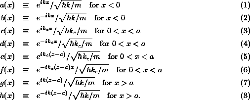
From our Schrödinger formulation, we know that the allowed solutions
to the TISE in the three regions (s), (c) and (t) of Figure
1 are forward and backward traveling plane waves with
wave vectors k, ![]() and k, where
and k, where ![]() and
and ![]() , respectively. We may generally
choose to represent these components of the final wave function as
, respectively. We may generally
choose to represent these components of the final wave function as
We have taken care to make each of our eight component solutions
![]() to carry unit current and to center each at an
appropriate point. We list two sets
of solutions c(x),d(x) and e(x),f(x) for region (c), as the
solutions in the corresponding region generally must satisfy boundary
conditions at the two end points, x=0 and x=a.
to carry unit current and to center each at an
appropriate point. We list two sets
of solutions c(x),d(x) and e(x),f(x) for region (c), as the
solutions in the corresponding region generally must satisfy boundary
conditions at the two end points, x=0 and x=a.
The first step in developing the Feynman rules is to agree upon a short-hand diagrammatic representation for all of these functions. Figure 2 shows these eight Feynman diagrams. Each time we draw one of these diagrams, it is meant to represent one of the eight functions (1-8). We may then use these diagrams rather than algebraic functions to write down equations.
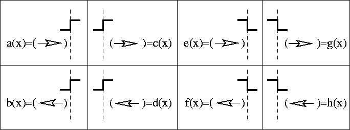
Figure 2: Eight Feynman Diagrams corresponding to the eight
solutions to the TISE ![]()
Two important equation relate c(x) to e(x) and d(x) to f(x). These pairs of functions represent the same physical state, a current flowing in Region (c) either to the right or left, respectively, and thus are related by a constant factors,
The complex exponential factor connecting these will appear so often in our analysis of scattering from this potential barrier that we give it a special name. As it represents the effect on the wave function of ``propagating'' across Region (c), we call the factor p for ``propagation,''
We now make our first diagrammatic equations. To represent (9) and (9) diagrammatically, we use the definitions from Figure 2 to produce the two diagrammatic equalities in Figure 3.
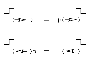
Figure: Diagrammatic Expression of Two Scattering Identities 9 and 10 (top
and bottom panels, respectively)