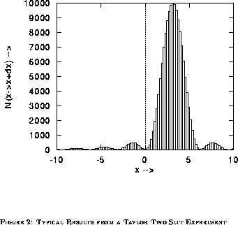
Mathematically, a random variable is defined as a quantity which may take a range of values with a given probability associated with each allowed value. This is closely related to the physical picture we have developed of an experiment. In G.I. Taylor's two slit experiment, where a single photon passes through the apparatus at a time, the arrival of each photon gives a separate measurement. The quantity which we measure in this case is the x coordinate of the spot indicating the location of the photon's arrival on the photographic plate. (See Figure 1.)

We customarily summarize the results of such an experiment in plot such as Figure 2. This plot tells how many measurements yielded values of x within each of the little bins (ranges in x) indicated in the plot.
We may idealize the situation to where the bins very narrow
and we wait long enough to record many photons in each bin. Then
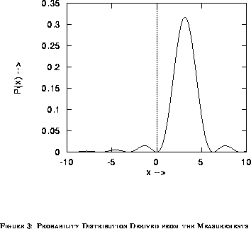
by normalizing the results by the total number of measurements
( ) made in the experiment (the total number of photons recorded) so
that
  gives the number of photons which arrived in
the range
  , we determine a probability
distribution which characterizes the experiment. (See Figure 3.)
Mathematically, we describe the experiment concisely with a random
variable X. We say that X is a random variable associated with
the position of the recording of the photons. X may take on any
value along the photographic plate (which for now we will imagine to
extend to  ) and the probability that it falls
in the range
  is just
  . X thus
describes the entire experiment whereas
  just represents the
arrival location of the photon in the experiment.
Note that it is also possible to have a random variable which takes on
only discrete values. In this case, we might have an experiment that
yields the values  . We would then say that the random
variable M takes the values
  with probabilities
 . All of the results we will demonstrate here are
valid for both continuous and discrete random variables. The proofs
for the discrete case involve the straight-forward replacement of
integrations with summations. We leave these proofs as an exercise to
the student.

